With much delight I’ve been following along on the fast.ai MOOC to get my feet wet with deep learning. Part 1, which focuses on getting started quick with cutting-edge techniques, was pretty wild, which motivated me to go on to Part 2. However, the pace changes with Part 2, and it’s more like an Area51 type deal. To quote Portal 2:
We’re throwing science at the wall here to see what sticks
Turns out some stuff sticks that would make Cave Johnson proud, but the learning curve is damn steep. You run into that head-first in Lecture 9 when it’s getting serious about multi-object detection in real time.
The problem
Jeremy, fast.ai’s lecturer, makes an honest attempt at introducing the theme slowly, but the terse code and myriad digressions into tangential topics (like why the code is terse) aren’t really helping. I found myself having to rewind so many times I can actually lip-sync to Jeremy while he is explaining the loss function part. I also have an unusually thick skull which doesn’t help when trying to understand a difficult topic.
The purpose of this post is to be able to explain to the version of me that existed 6 days ago, what SSD is about, in plain English (assuming some prior Deep Learning knowledge). With that fairly intuitive foundation in mind, the lecture should be easier to grasp. I’m not going to go into hairy technical details, that’s just going to distract from the intuitive understanding. I’m planning on getting more into that in a later post.
The below explanation is slightly specific for SSD, but let’s be real, it’s so top-level you could also interpret it for the YOLO architecture.
Single Shot Multibox Detector
The general idea of SSD is this: we’re going to start with a pre-existing convolutional net that can already “see” (the SSD paper uses pre-trained VGG16, Jeremy uses ResNet34). By “see” I mean that it can reliably classify real-world objects like cars, planes, cats, dogs etc.
On top of this “backbone” network, we are going to put an SSD “head”, which will spit out coordinates of bounding boxes and what classes the network thinks those boxes contain. It will do this based on successive convolutional layers built on top of the “backbone” network.
Woah, hold the phone, “boxes”?
The idea is actually fairly simple. Let’s say you’re a convolutional network, and you can already “see”. Now I want you go to the next level, and tell me the coordinates of boxes in the picture that contain the “objects” you’re recognising.
Right now though, that’s a bit of a stretch: you’ve been trained to classify images, sure, but conjuring up coordinates out of thin air, that’s a tall order, especially if there’s multiple objects/boxes.
No problem, I’ll help you out: I’ll just feed you a pre-defined list of boxes (we call these “anchor boxes”) you can use. All you have to do is shift them around a little, or maybe scale them a bit, so that they contain whatever is in the vicinity of that box. Oh, and I’ll need you to tell me what the class is of the object is you’ve got in those boxes.
Loss Function
So how will I tell whether you are doing a good job at spitting out bounding boxes? It’s a fairly straightforward process that works in two stages. The first stage is more commonly referred to as the “matching stage”.
Stage 1
During the matching stage, I will go through all of the boxes that you’re outputting, and calculate their overlap with the ground truth boxes I have. The metric I’ll use for this is called the Jaccard Index (a.k.a. IOU). If the Jaccard Index is lower than 0.5, I’ll ignore this prediction completely. This makes intuitive sense: how can I grade your predictions if there is no ground truth to compare it against?
Stage 2
If the Jaccard Index is larger than 0.5 though, that means there was a “match”, and I’ll move to the second stage. Here, I’ll grade your prediction on two parts:
- I’ll calculate the L1 loss of the coordinates you predicted, and reward you if you find a way to tweak (read: backprop) your algorithm to lower that loss (i.e. make the overlap bigger)
- Additionally, I’ll take a look at the class you predicted for that box, and reward you if you can find a way to tweak your algorithm to get the right class and be confident in it (Binary Cross Entropy loss, that’s standard stuff you’ve seen for multi-class classification in Part 1)
That’s it really.
More on Anchor Boxes
Honestly, when you first get in touch with them, this concept of anchor boxes is a bit confusing. Especially because in the initial examples, there seems to be no difference between anchor boxes and simple grid cells. Try to think of anchor boxes as a pre-defined list of boxes that could actually have any shape, and are just there to help the algorithm on its way. They’re initially the same as grid cells because, I don’t know, seems a good a place as any to start.
However, you’ll notice Jeremy doesn’t stick to vanilla boxes for long. When he’s talking about “More anchor boxes!” around the 2:05:00 mark, you’ll notice he starts kind of augmenting them, by changing their aspect ratio and size. It’s to help the algorithm even more!
How is that? Remember: the algorithm can only change the boxes a little. We help it along by not only feeding it standard, square, grid-cell type boxes, but also their deformed variants! This will later tie in to the factor k you can see floating around the SSD architecture code.
Object Sizes
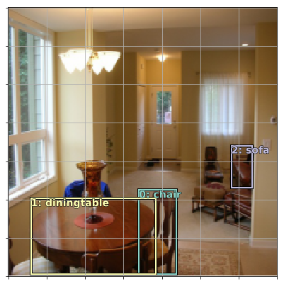
But wait, there’s more! Let’s imagine you have a picture, and we’ve segmented it into a 4x4 grid. As covered above, we’ll turn that grid into 16 anchor boxes, maybe do some augmentation, and feed them to the algorithm. Cool.
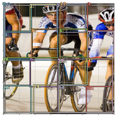
But what if there is an object in that picture, like the cyclist below, that takes a whole 2x4 space? There is just no way the algorithm can can “tweak” just one of the tiny 16 anchor boxes to fit the whole cyclist, not even if we help it with augmentation.
Thankfully, as we covered above, SSD does convolutions. So here’s what we’ll do in the SSD head:
- We’ll have a convolutional layer that uses a 4x4 grid, and have it output bounding boxes and classes
- But we’ll also take that 4x4 layer and put it through a
Conv2Dwith stride 2. This leads us to a 2x2 grid. Here again, we’ll have it spit out bounding boxes and classes - Then we’ll do it again! One
Conv2Dstride 2 later, we end up with a 1x1 grid, which again spits out bounding boxes and classes
If you think it through, you’ll agree that at the 4x4 resolution, one of those 16 boxes just can’t be stretched up enough to fit the 2x4 cyclist. Remember, our algorithm can only make minor tweaks to the anchor boxes we propose. However, maybe one of the 4 boxes in the 2x2 layer could fit the object, if the algorithm scales it juuust right. And even if those are too small, it’s certain that we can just take the 1x1 box (which by definition covers the whole image) and scale it decently to fit the cyclist.
That’s how we can leverage the multiple convolutional layers of the SSD head to give us bounding boxes at different “resolutions”, so we can detect small objects as well as large ones.
Wrapping Up
I can’t believe how long this post ended up being, while I was trying to stick to plain English. SSD, and generally single shot detection is insanely cool, but it takes quite some thinking to really grasp all the moving parts. Hope this was useful. Still have questions? Check out the forum over at forums.fast.ai for some of the best deep learning communities the internet has to offer.
What’s with the “single shot” stuff though
The “single shot” (or “once” in the YOLO name), mean that you only feed the image once through the entire integrated network (one single forward pass). That’s different from previous state of the art, which usually had multiple stages that explicitly specialised in different aspects of solving the problem.
Thanks to Radek for proof-reading!